Clock/model visualizations using GEO datasets

This example demonstrates the built-in aging clock/model function to visualize different plots on clock(s)/model(s) predictions.

Import required classes and functions

from biolearn.data_library import DataLibrary
from biolearn.model_gallery import ModelGallery
from biolearn.visualize import (
    plot_clock_correlation_matrix,
    plot_clock_deviation_heatmap,
    plot_age_prediction,
    plot_health_outcome
)

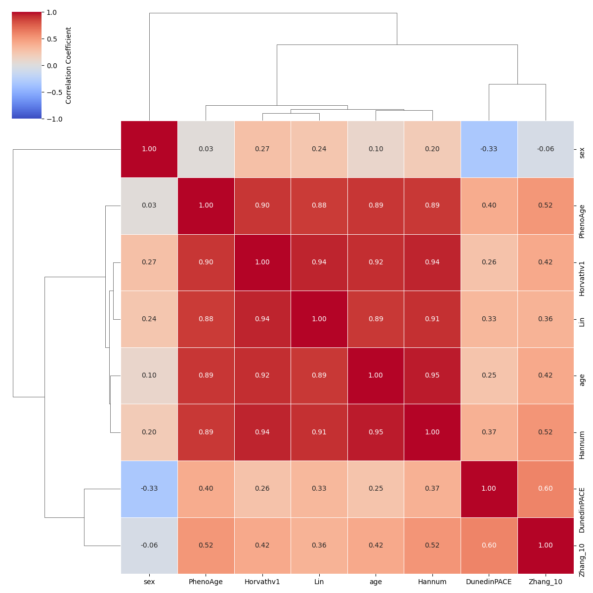
Visualize a correlation matrix across aging clocks/models

# Load an appropriate GEO dataset for the models
data = DataLibrary().get("GSE120307").load()

# Create a list of ModelGallery objects to be analyzed.
modelnames = ["Horvathv1", "Hannum", "PhenoAge", "DunedinPACE", "Lin", "Zhang_10"]
models = [ModelGallery().get(names) for names in modelnames]

plot_clock_correlation_matrix(
    models=models,
    data=data,
)

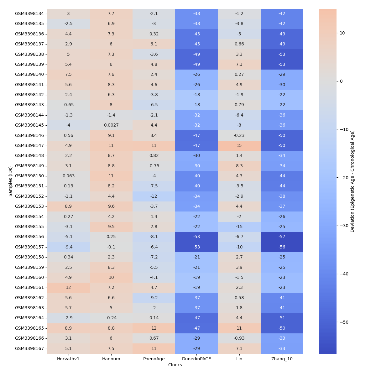
Visualize clock/model chronological age deviations across samples in a heatmap

plot_clock_deviation_heatmap(
    models=models,
    data=data,
)

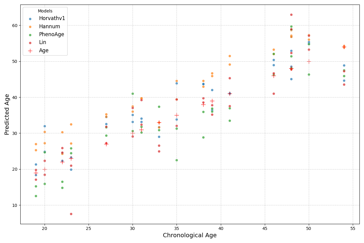
Visualize aging clock/model predictions against chronological age

# Use appropriate clocks/models
modelnames = ["Horvathv1", "Hannum", "PhenoAge", "Lin"]
age_prediction_models = [ModelGallery().get(name) for name in modelnames]

plot_age_prediction(
    models=age_prediction_models,
    data=data,
)

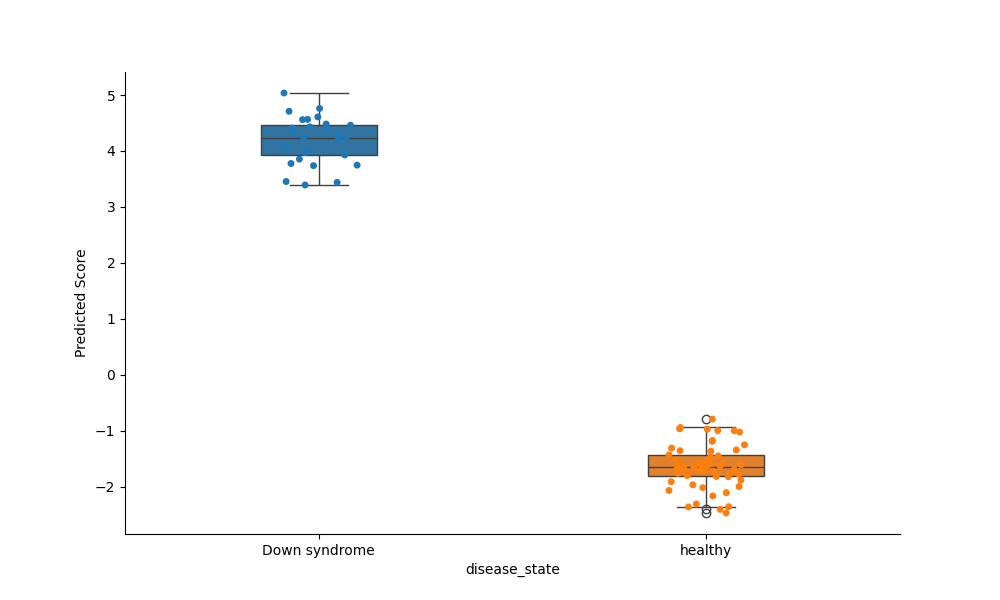
Visualize model predictions against its corresponding health outcome

# Load an appropriate GEO dataset for the corresponding model
down_syndrome_data = DataLibrary().get("GSE52588").load()

model = [ModelGallery().get("DownSyndrome")]

plot_health_outcome(
    models=model,
    data=down_syndrome_data,
    # Provide the health outcome column name
    health_outcome_col="disease_state",
)

Estimated memory usage: 1483 MB