Exploring the Challenge Data#

This example shows you how to load and explore the challenge data with biolearn

Loading up the data for the competition#

from biolearn.data_library import DataLibrary

challenge_data = DataLibrary().get("BoAChallengeData").load()

The challenge data has methylation data#

GSM7866999 GSM7867305 GSM7867077 ... GSM7867431 GSM7867126 GSM7867000
cg00000029 0.720084 0.453491 0.535564 ... 0.487361 0.337215 0.062426
cg00000109 0.938044 0.925149 0.949446 ... 0.938523 0.940187 0.942090
cg00000155 0.957093 0.959030 0.948919 ... 0.966912 0.968026 0.970274
cg00000158 0.965191 0.957272 0.967278 ... 0.971039 0.969745 0.969660
cg00000165 0.144061 0.122099 0.167346 ... 0.156199 0.133038 0.641788
... ... ... ... ... ... ... ...
rs9292570 0.523412 0.980810 0.986609 ... 0.525876 0.537722 0.538440
rs9363764 0.960815 0.038638 0.451884 ... 0.978343 0.971838 0.973633
rs951295 0.971034 0.558011 0.553397 ... 0.485287 0.526686 0.499980
rs966367 0.455920 0.963994 0.453094 ... 0.455700 0.029342 0.026907
rs9839873 0.599735 0.595571 0.630871 ... 0.576566 0.579195 0.973815

930659 rows × 500 columns


The challenge data also has proteomic data#

GSM7867173 GSM7867127 GSM7867083 ... GSM7867095 GSM7867115 GSM7867385
AlamarTargetID
t10319 13.387778 12.948052 13.256551 ... 12.062449 13.390582 13.587867
t10413 16.674015 15.992939 15.547946 ... 14.827118 15.872686 15.584386
t10466 12.890963 13.556167 13.528756 ... 14.683530 13.667331 13.483932
t10563 10.933342 8.323690 13.271350 ... 9.993500 11.699095 11.860206
t10876 14.063506 15.429302 13.582464 ... 11.978461 6.654607 11.931614
... ... ... ... ... ... ... ...
t8333 14.725785 13.537733 14.848917 ... 13.729721 13.787099 14.055526
t8334 13.503408 12.103376 13.381374 ... 13.070087 14.317681 14.314627
t8358 12.734120 15.238780 11.673970 ... 13.103683 13.949114 13.794795
t8367 11.062422 12.291734 12.604654 ... 11.803189 14.313347 13.830717
t8399 11.599597 14.642498 14.590723 ... 12.073775 14.184558 12.040475

374 rows × 503 columns


You can learn more about what the protein identifies in our reference#

from biolearn.util import get_data_file

reference = pd.read_csv(get_data_file("reference/alamar_reference.csv"))
reference
AlamarTargetID UniProtID Target ProteinName
0 t10034 O75888 TNFSF13 TNF superfamily member 13
1 t10319 O95760 IL33 Interleukin 33
2 t10412 P01258 CALCA Calcitonin [Cleaved into: Calcitonin; Katacalcin
3 t10417 P01903 HLA-DRA Major histocompatibility complex, class II, DR...
4 t10433 P02745 C1QA Complement C1q A chain
... ... ... ... ...
317 t8244 P35247 SFTPD Pulmonary surfactant-associated protein D
318 t8246 P22303 ACHE Acetylcholinesterase
319 t8254 Q8N474 SFRP1 Secreted frizzled-related protein 1
320 t8355 P0DJI8 SAA1 Serum amyloid A-1 protein
321 t9441 O15240 VGF VGF nerve growth factor inducible

322 rows × 4 columns


Some of the data overlaps while some does not but all the metadata is combined#

age sex subject_id tissue
GSM7866964 31.35 2 BoA1 Blood
GSM7866965 79.45 1 BoA2 Blood
GSM7866966 60.42 2 BoA3 Blood
GSM7866967 59.24 1 BoA4 Blood
GSM7866968 22.41 1 BoA5 Blood
... ... ... ... ...
P499 80.98 1 NaN NaN
P500 89.00 1 NaN NaN
P501 80.92 2 NaN NaN
P502 69.80 1 NaN NaN
P503 68.18 1 NaN NaN

651 rows × 4 columns


You can easily run several models on them#

from biolearn.mortality import run_predictions

prediction_dict = {
    "Horvathv1": "Predicted",
    "Hannum": "Predicted"
}

predictions = run_predictions(challenge_data, prediction_dict)
predictions
Horvathv1 Hannum
GSM7866999 21.822423 17.303025
GSM7867305 56.266752 52.803410
GSM7867077 39.660930 36.211078
GSM7867095 29.806215 32.821235
GSM7867457 51.285108 49.308239
... ... ...
GSM7867136 37.539954 32.494127
GSM7867452 74.975617 68.639608
GSM7867431 33.083565 33.906176
GSM7867126 91.428559 74.870807
GSM7867000 75.005273 77.630528

500 rows × 2 columns


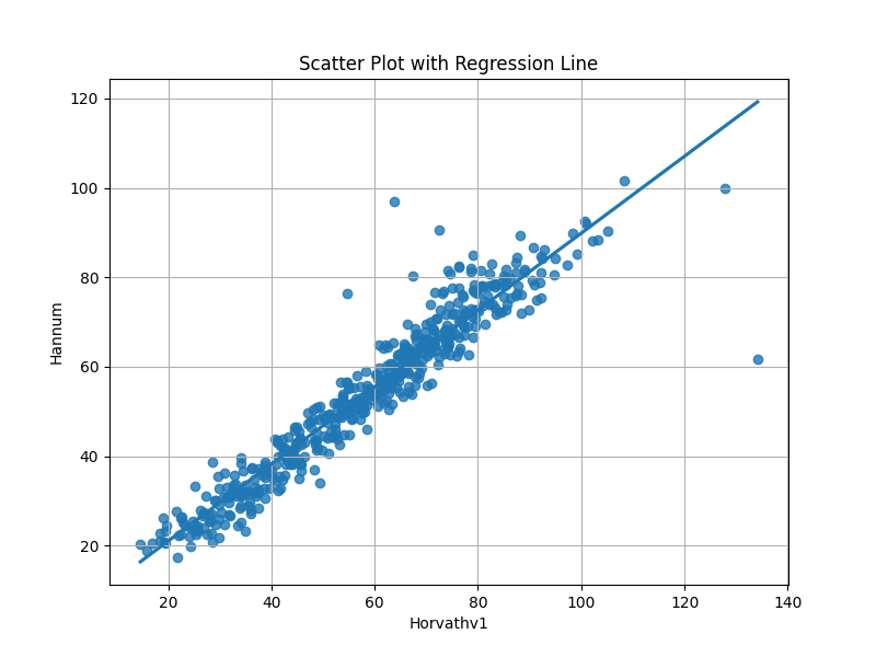
We can then compare the output from the two models#

import matplotlib.pyplot as plt
import seaborn as sns

# Assuming your dataframe is named 'df'
# df should have columns 'Horvathv1' and 'Hannum'

# Create a scatter plot with a regression line
plt.figure(figsize=(8, 6))
sns.regplot(x='Horvathv1', y='Hannum', data=predictions, ci=None)

plt.title('Scatter Plot with Regression Line')
plt.xlabel('Horvathv1')
plt.ylabel('Hannum')
plt.grid(True)
plt.show()
Scatter Plot with Regression Line

Total running time of the script: (0 minutes 20.893 seconds)

Estimated memory usage: 15052 MB

Gallery generated by Sphinx-Gallery