“Epigenetic Clocks” in GEO Data

This example loads a DNA Methylation data from GEO, calculates multiple epigenetic clocks, and plots them against chronological age.

First load up some methylation data from GEO using the data library

from biolearn.data_library import DataLibrary
#Load up GSE41169 blood DNAm data
data_source = DataLibrary().get("GSE41169")
data=data_source.load()

Now run three different clocks on the dataset to produce epigenetic clock ages

from biolearn.model_gallery import ModelGallery
gallery = ModelGallery()
#Note that by default clocks will impute missing data.
#To change this behavior set the imputation= parameter when getting the clock
horvath_results = gallery.get("Horvathv1").predict(data)
hannum_results = gallery.get("Hannum").predict(data)
phenoage_results = gallery.get("PhenoAge").predict(data)

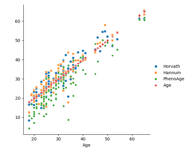
Finally extract the age data from the metadata from GEO and plot the results using seaborn

import seaborn as sn
import pandas as pd

actual_age = data.metadata['age']
plot_data = pd.DataFrame({
    'Horvath': horvath_results['Predicted'],
    'Hannum': hannum_results['Predicted'],
    'PhenoAge': phenoage_results['Predicted'],
    "Age": actual_age
})
plot_data.index=plot_data['Age']

sn.relplot(data=plot_data, kind="scatter");

<seaborn.axisgrid.FacetGrid object at 0x724f34ea4970>

Estimated memory usage: 1704 MB